Viewing Language Through a Probabilistic Lens

Genisis

Humans gain semantic and syntactic meaning through repeated exposure to language and context. Models, on the other hand, get a different kind of exposure, with no exact mapping of what a word semantically represents in a sentence.

The paradigm of large language models has evolved meaningfully, but some of the primitives remain the same. This blog is a fundamental building piece toward the question: “How can semantics emerge from a system trained only to predict symbols?”

The starting point for this exploration is A Neural Probabilistic Language Model (2003).

The problem with n-gram models

Understanding the n-gram model:

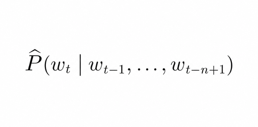
An n-gram model is a finite-context probabilistic language model that approximates the probability of the next token using only the previous $(n-1)$ tokens.

According to the experiment done in the paper, various n-gram models performed realtively well on a larger corpus than on the smaller ones.

Question: Why don’t we just scale the corpus during training?

The answer is that scaling the corpus helps, but it does not solve the underlying problem.

Think about a corpus with vocabulary size:

$$V=100,000$$

If the model needs to determine the joint distribution of 10 consecutive words, there are potentially:

$$100,000^{10}-1=10^{50}-1$$

free parameters.

As the context grows, the number of possible word sequences grows exponentially. A realistic corpus can only cover a tiny fraction of them, meaning most contexts will either be unseen or too rare to estimate reliably.

This phenomenon is called the curse of dimensionality.

The missing notion of similarity

Think about the two words “Homo sapiens” and “human”. We know that these two terms are semantically very close and can occupy similar roles in a sentence, but for a counting model they are still two separate arbitrary symbols.

Meaning, if the sentence “I am a human.” appears in the training corpus 10 times but “I am a Homo sapiens.” does not appear even once, the model does not inherently transfer what it learned from human to Homo sapiens.

Learning a distributed representation for words

The solution proposed in the paper to the very problem mentioned in the last section is to stop treating words only as arbitrary discrete symbols.

Each word in the vocabulary is mapped to a real-valued vector:

$$C(i)\in {\mathbb{R}}^m$$

where $C$ is a matrix containing the representation of every word in the vocabulary, and $C(i)$ is the representation of word $i$.

For a context containing multiple words, their representations are concatenated into:

$$x=(C(w_{t-1}),C(w_{t-2}),\dots ,C(w_{t-n+1}))$$

This changes the problem from operating directly on discrete word identities to operating on points in a continuous space.

But the important part is that the values inside $C$ are not determined beforehand. They are free parameters of the model and are learned together with the probability function.

The model starts with randomly initialized word representations. Those representations are used to predict the next word. The prediction produces an error, and that error is backpropagated through the network into the specific rows of $C$ that were used as input.

In other words:

word → C(word) → probability model → prediction → error → update C(word)

This process repeats across the training corpus.

So the representation of a word is shaped by the predictions that word helps the model make. If two words repeatedly occur in contexts where they need to support similar predictions, their vectors can gradually acquire similar structure.

No semantic relationship between those words is explicitly provided to the model. The structure in $C$ emerges because that structure becomes useful for predicting language.

What if we stopped at distributed representation?

At this point, we have given words a better representation.

A word is no longer just an arbitrary discrete symbol. It now exists as a learned vector inside $C$, and words that are useful in similar contexts can acquire similar representations.

But that still does not give us a language model.

Knowing that human and Homo sapiens are close in the representation space does not tell us whether the next word after:

I am a

should be human, student, developer, or something else.

Distributed representation solves how words are represented.

It does not yet solve how those representations become a prediction.

So we need another function on top of them.

Turning context into a useful signal

The model is not predicting from a single word. It is predicting from a context.

$C$ contains the learned representation of every word in the vocabulary, but for one prediction we only need the rows corresponding to the current context.

So if the context is:

the cat is

we take:

$C(\text{the})$, $C(\text{cat})$, and $C(\text{is})$

and concatenate them into one vector:

$$x=(C(w_{t-1}),C(w_{t-2}),\dots ,C(w_{t-n+1}))$$

Here, $x$ is simply the context vector, the current context represented using the learned word vectors from $C$.

Now imagine again:

the cat is

Each word contributes information, but the useful signal may exist in the combination of those words rather than in any one vector independently.

We therefore transform $x$:

$$d+Hx$$

$H$ is a learned weight matrix. Its job is to combine the different features present in the context.

$d$ is a bias, a learned offset added before the next transformation.

But if we only used matrix multiplication and addition, the relationship would still be linear. We would be limited in the kinds of interactions we could represent.

So we apply:

$$\tanh (d+Hx)$$

$\tanh$ is a non-linear activation function. In simple terms, it lets combinations of features behave differently rather than forcing every relationship to remain a straight linear transformation.

The result is what we call the hidden representation: the context after it has been transformed by $H$, $d$, and $\tanh$.

At this stage, we have something more useful than the raw concatenated vectors, but we still do not have a prediction.

Turning the signal into probability

The hidden representation now needs to influence every possible next word.

We do that using:

$$U\tanh (d+Hx)$$

$U$ is another learned weight matrix. It takes the hidden representation and maps it into one score for every word in the vocabulary.

If the vocabulary contains 10,000 words, this operation produces 10,000 scores.

There is also an optional direct path:

$$Wx$$

$W$ is a shortcut from the original context vector directly to the output scores.

This means the model can learn through two routes:

x → W → output

x → H → tanh → U → output

The hidden path can capture more complex non-linear interactions.

The direct path can preserve simpler relationships that do not need to pass through the hidden transformation.

We also add an output bias $b$, another learned offset, which gives each vocabulary word its own baseline preference.

Everything comes together here:

$$y=b+Wx+U\tanh (d+Hx)$$

$y$ is now a vector containing one score for every possible next word.

These scores are called logits.

A logit is simply an unnormalized score. A larger logit means the model currently favors that word more, but logits are not probabilities yet. They can be negative, positive, and they do not need to sum to one.

So we need one final operation.

Softmax

Softmax takes all the logits and turns them into a probability distribution:

$$\hat{P}(w_t\mid w_{t-1},\dots ,w_{t-n+1})=\frac{e^{y_{w_t}}}{{\sum }_i{e}^{y_i}}$$

The numerator exponentiates the score of the candidate word.

The denominator does the same for every possible word and sums them together.

Dividing by that total normalizes the scores so that all final probabilities add up to 1.

So if walking receives a much larger logit than blue, softmax gives walking a much larger probability.

Now the full path becomes:

context words
→ rows from C
→ concatenate into x
→ transform with H and tanh
→ map to vocabulary scores with U
→ optionally add the direct Wx path
→ add bias b
→ logits y
→ softmax
→ P(next word | context)

The Limitation

We have established that each word is represented as a single point in the vector space. This is one of the biggest limitations of the model when it comes to generalization. Before answering why, think about what information gets lost when one word is forced into one fixed representation.

…

Fundamentally, a single word may represent different meanings depending on its context. If that word is represented by only one vector, all of those meanings are compressed into the same representation.

Take the word bank.

I deposited money in the bank.

We sat by the river bank.

The symbol is identical, but its meaning is not. A single static representation cannot fully distinguish between those two contextual meanings.

The second major limitation of this approach was computation. The output layer requires scores to be computed across the vocabulary, which made training extremely expensive as the vocabulary grew.

I highly suggest reading the actual paper for this part, especially Section 3: Parallel Implementation and the experimental discussion in Section 4.

Final Notes

Large Language Models are often referred to as “next token predictors”. Building gpt-from-first-principles and writing Working with Text Data had given me a premature understanding of what that actually meant.

Reading A Neural Probabilistic Language Model gave that phrase much more depth.

I had already seen the mechanics of token prediction. What I had not understood was why learning to predict the next word could also force the model to learn useful representations of language.

Let’s build the intuition, paper by paper.